Mathematical methods for baselinenowcast
Source:vignettes/model_definition.Rmd
model_definition.RmdOverview
The baselinenowcast model is based on the reference model for the COVID-19 hospital admissions nowcasting challenge in Germany in 2021 and 2022[1]. Using a slight variation of the chain ladder method[2], the method uses preliminary case counts and empirical delay distributions to estimate yet-to-be-observed cases. Probabilistic nowcasts are generated using an observation model with means from the point nowcast and uncertainty estimated from past nowcast errors. Users can flexibly specify the data they would like to use for delay estimation and uncertainty quantification, as well as specify the parametric form of the observation model used for uncertainty quantification. Time steps can correspond to any time unit. See the Default Settings section for a full description of the default behaviour of the baselinenowcast() method.
Notation
We denote \(X_{t,d}, d = 0, \dots, D\) as the number of cases occurring at time \(t\) which appear in the dataset with a delay of \(d\). For example, a delay \(d = 0\) means that a case occurring on day \(t\) arrived in the dataset on day \(t\). We only consider cases reporting within a maximum delay \(D\). The number of cases reporting for time \(t\) with a delay of at most \(d\) can be written as:
\[ X_{t, \le d} = \sum_{i=0}^d X_{t,i} \tag{1} \]
A special case of this is the “final” number of reported cases at time \(t\), denoted by \[ X_t = X_{t, \le D} = \sum_{i=0}^D X_{t,i} \]
For delays \(d < D\) we define the notation
\[X_{t,>d} = \sum_{i = d+1} ^{D} X_{t,i}\]
representing the number of cases still missing after \(d\) delay. In the following we use uppercase letters (\(X_t\)) for random variables, lower case (\(x_t\)) for the corresponding observations, and hats (\(\hat{x}_t\)) for estimated/imputed values. We refer to \(X_t\) to describe a random variable, \(x_t\) for the corresponding observation, and \(\hat{x}_t\) for an estimated/imputed value. The matrix \(\mathbf{x}\) with entries \(x_{t,d}, t = 1, \dots, t^*, d = 1, \dots, D\) is referred to as the reporting matrix. For a description of the nowcasting terms being used in this document (e.g. reporting triangle) and their corresponding abbreviations in the package, please consult the nowcasting nomenclature vignette.
| \(d = 0\) | \(d = 1\) | \(d=2\) | \(...\) | \(d= D-1\) | \(d= D\) | |
|---|---|---|---|---|---|---|
| \(t=1\) | \(x_{1,0}\) | \(x_{1,1}\) | \(x_{1,2}\) | \(...\) | \(x_{1,D-1}\) | \(x_{1, D}\) |
| \(t=2\) | \(x_{2,0}\) | \(x_{2,1}\) | \(x_{2,2}\) | \(...\) | \(x_{2,D-1}\) | \(x_{2, D}\) |
| \(t=3\) | \(x_{3,0}\) | \(x_{3,1}\) | \(x_{3,2}\) | \(...\) | \(x_{3,D-1}\) | \(x_{3, D}\) |
| \(...\) | \(...\) | \(...\) | \(...\) | \(...\) | \(...\) | \(...\) |
| \(t=t^*-1\) | \(x_{t^*-1,0}\) | \(x_{t^*-1,1}\) | \(x_{t^*-1,,2}\) | \(...\) | \(x_{t^*-1,,D-1}\) | \(x_{t^*-1,D}\) |
| \(t=t^*\) | \(x_{t^*,0}\) | \(x_{t^*,1}\) | \(x_{t^*,2}\) | \(...\) | \(x_{t^*,D-1}\) | \(x_{t^*, D}\) |
In the case where \(t^*\) corresponds to the present date, all entries with \(t+d>t^*\) have yet to be observed and are thus still missing. As the available entries at its bottom form a triangle, this incomplete reporting matrix is referred to as the reporting triangle.
| \(d = 0\) | \(d = 1\) | \(d=2\) | \(...\) | \(d= D-1\) | \(d= D\) | |
|---|---|---|---|---|---|---|
| \(t=t^*-2\) | \(x_{t^*-2,0}\) | \(x_{t^*-2,1}\) | \(x_{t^*-2,2}\) | \(...\) | ||
| \(t=t^*-1\) | \(x_{t^*-1,0}\) | \(x_{t^*-1,1}\) | \(...\) | |||
| \(t=t^*\) | \(x_{t^*,0}\) | \(...\) |
Pre-processing of the reporting triangle
All of the following steps require that the reporting triangle only has non-negative entries. In practice this is not necessarily the case. For instance, if the reporting triangle has been computed from increments in subsequent data snapshots, occasional downward corrections due to data entrance issues can cause negative entries. We therefore apply a pre-processing step to re-distribute negative entries across neighbouring cells with positive entries.
Delay distribution estimation
Estimating the delay distribution from a reporting matrix
If a complete reporting matrix is available, estimating the discrete-time delay distribution \(\pi_d, d = 0, \dots, D\) is straightforward. Using the last \(N\) rows of the reporting matrix \(\mathbf{x}\), we compute
\[ \hat{\pi}_d= \frac{\sum_{t=t^*-N+1}^{t=t^*} x_{t,d}}{\sum_{t=t^*-N+1}^{t=t^*} x_{t}}, \tag{2} \] which is simply the relative frequency of a delay of \(d\) days among all cases in the reporting matrix.
Estimating the delay distribution from a reporting triangle
In the case where \(t^*\) is the present day, such that only a reporting triangle with missing entries is available, the estimator \(\hat{\pi}_d\) from (2) can only be evaluated after discarding all data from the last \(D-1\) time points. In order to use these partial observations, we use a different representation of the delay distribution via terms of the form
\[ \theta_d = \frac{\pi_d}{\pi_{\le d-1}} \tag{3} \]
for \(d = 1, \dots, D\). Here, in analogy to (1) we write
\[ \pi_{\le d-1} = \sum_{d'=0}^{d-1} \pi_d. \tag{4} \]
The \(\theta_d\) can be estimated via
\[ \hat{\theta}_d = \frac{\sum_{t=t^* - N + 1}^{t^*-d} x_{t, d}}{\sum_{t= t^* - N + 1}^{t^*-d} x_{t, \leq d - 1}}, \]
and translated to estimates \(\hat{\pi}_0,..., \hat{\pi}_D\) via the recursion
\[ \hat{\pi}_{\leq d} = (1+\hat{\theta}_d)\hat{\pi}_{\leq d-1} \]
subject to the constrain that \(\sum_{d = 0}^D \pi_d = 1\).
We note that this method is equivalent to the so-called chain ladder method[2], adapted to our notation in terms of reporting triangles (rather than development triangles as used in accounting). The intuition behind the method relies on the basic assumption is that the ratio between the delays in the complete observations is equivalent to the ratio between the delays in the partially observed components of the matrix (Figure 1).
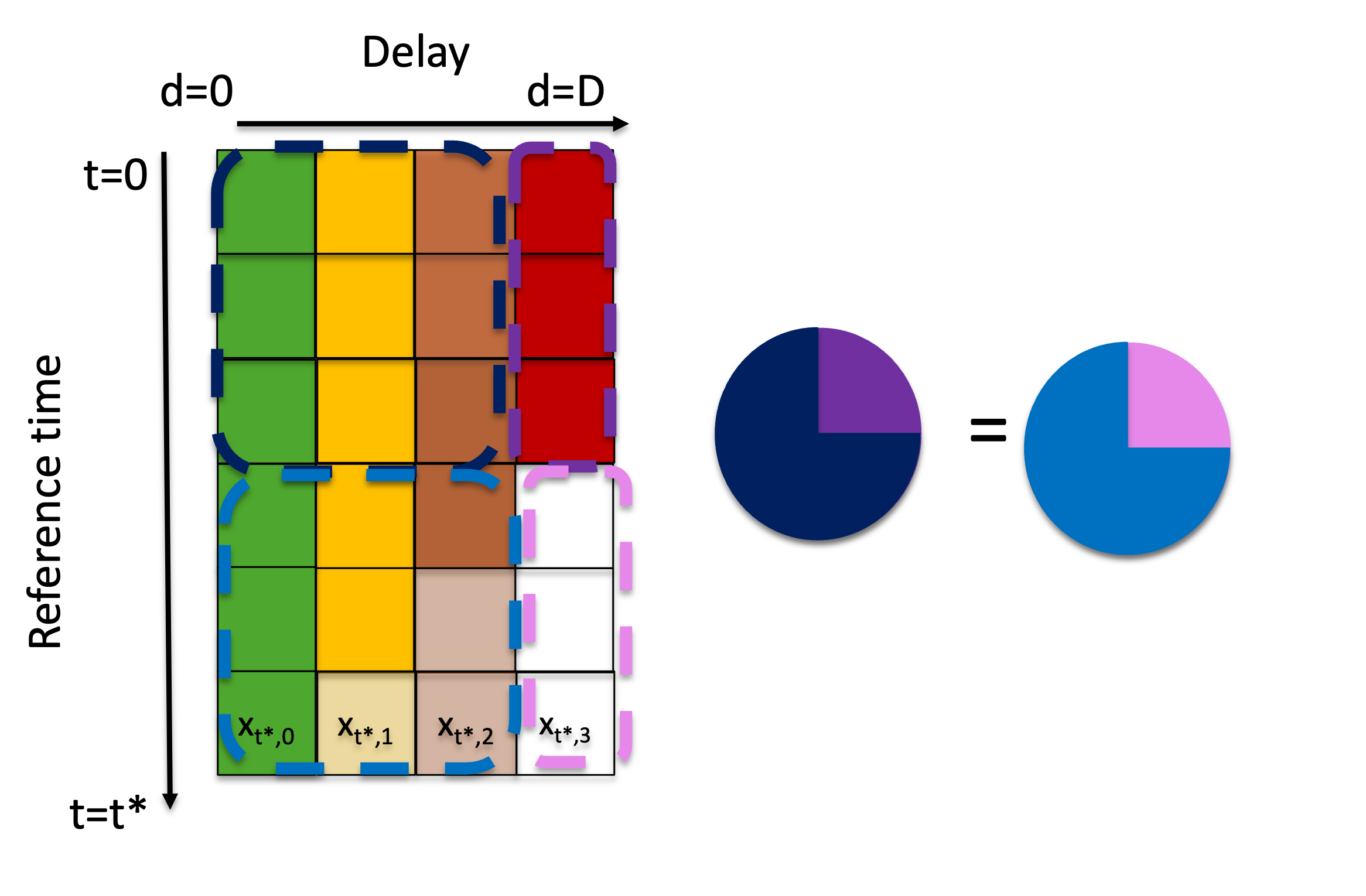
Figure 1: Visual description of the iterative “completing” of the reporting triangle, which relies on the assumption that the ratio between delays for fully observed reference times is consistent with the ratio between those same delays in the partially observed data.
The delay_estimate() function ingests either a reporting matrix or a reporting triangle and uses the last n rows to compute an empirical delay probability mass function (PMF), returning a simplex vector indexed starting at delay 0.
Point nowcast generation
We now address the computation of a point nowcast, i.e., expected final case numbers \(\hat{x}_t, t = t^* - D + 1, t^*\). These are based on the reporting triangle, more specifically the preliminary totals \(x_{t, \leq t^* - t}\), and the estimated delay distribution, \(\hat{\pi}_d, d = 0, \dots, D\). In the following we will denote the current time \(t^*\) as the nowcast time, and the time \(t = t^* - D, \dots, t^*\) as the reference time. The difference \(j = t^* - t\) will be called the horizon.
An intuitive approach, used in[1] and the standard chain ladder technique, is to simply inflate the current total for a reference time \(t\) by the inverse of the respective probability of observation up to time \(t^*\),
\[ \hat{x}_t =\frac{x_{t, \leq t^*-t}}{\pi_{\leq t^*-t}}. \]
This, however, is not well-behaved if no cases at \(t\) have been observed yet, i.e., \(x_{t, \leq t^* - t} = 0\). Then \(\hat{x}_t\) is likewise zero, which yields problems in our uncertainty quantification method (see next section). Motivated by a Bayesian argument (see Zero-handling below) we therefore use the expression
\[ \hat{x}_t = \frac{x_{t, \leq t^*-t} + 1 - \pi_{\leq t^*-t}}{\hat{\pi}_{\leq t^*-t}} \tag{5} \]
instead. This yields essentially identical results for large \(x_{t, \leq t^* - t}\), but produces positive \(\hat{x}_t\) even for preliminary zero values \(x_{t, \leq t^* - t} = 0\).
For our uncertainty quantification scheme we require not only estimated totals \(\hat{x}_t\), but all entries \(\hat{x}_{t,d}\) of a point nowcast matrix. For \(t = t^* - D + 1, \dots, t^*, d > t^* - t\) these are obtained as
\[ \hat{x}_{t,d} = \hat{\pi}_d \times \hat{x}_t. \]
The apply_delay() function ingests a reporting triangle and a delay PMF and returns a point nowcast matrix by “filling in” the missing elements of the reporting triangle.
The generation of a point nowcast is described in the schematic below (Figure 2), demonstrating how the missing elements of the reporting triangle are estimated and can then be used to generate a point estimate of the final counts at each reference time.
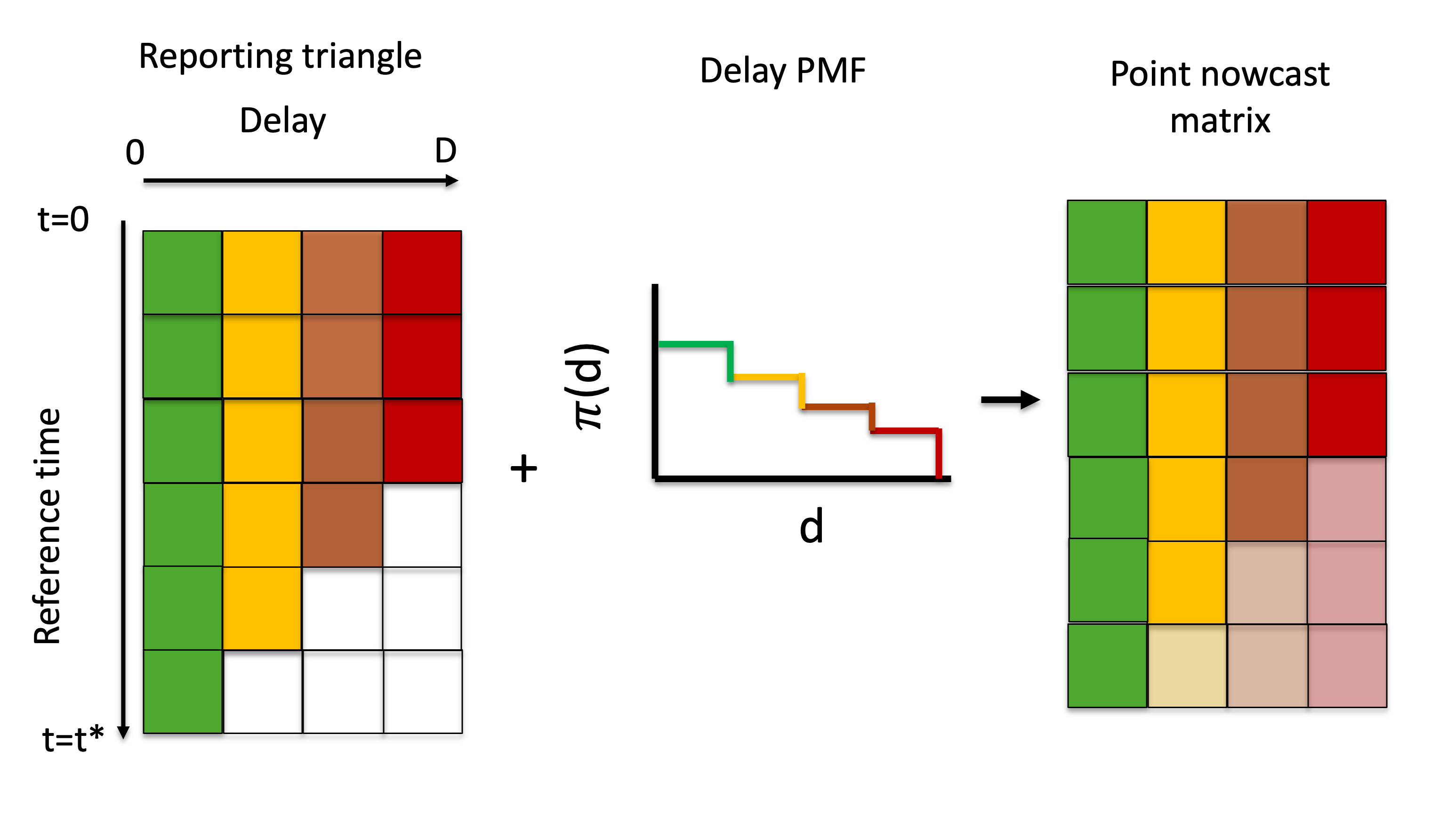
Figure 2: Visual description of the generation of a point nowcast matrix from a reporting triangle and delay PMF.
Uncertainty quantification
To estimate the uncertainty in the nowcasts, we use the nowcast errors from \(M\) past nowcasting time points. See the Default Settings for more details on the default settings used in the package to define the number of \(M\) past nowcasting time points used.
Generation of retrospective reporting triangles
We first obtain “vintage” reporting triangles of the raw reporting triangle (i.e., before pre-processing) to replicate the data which would have been available as of times \(s^* = t^*-1, ..., t^*-M\), i.e., the last \(M\) time points on which nowcasts could have been generated. This simply corresponds to the stepwise omission of all entries with \(t + d > s^*\), which for each \(s^*\) is a diagonal from the bottom left to the top right. The same pre-processing step as in Section Preprocessing of the reporting triangle is applied to each vintage reporting triangle.
This can be achieved in a stepwise manner using the functions truncate_to_rows() and apply_reporting_structure() which return a list of n retrospective reporting triangles in order from most recent to oldest.
Generation of retrospective point nowcast matrices
For each of the \(M\) vintage reporting triangles, i.e., \(s^* = t^*-1,, ..., t^*-M\), we apply the method described above to estimate a delay distribution and generate a point nowcast matrix using the function estimate_and_apply_delays().
To indicate the data version on which it is based, its entries are denoted by:
\[ \hat{x}_{t, d}(s^*) \]
for \(t = s^* - D + 1, \dots, s^*\) and \(d = s^* - t + 1, \dots D\).
Note that estimation is again based on the last \(N\) rows of the respective reporting triangle, which must consequently contain at least \(M + N\) rows in total.
Fit an observation model to past nowcast errors
A point nowcast based on the reporting triangle from time \(s^*\) can also be written as
\[ \hat{x}_{t}(s^*) = x_{t, \leq s^* - t} + \hat{x}_{t, > s^* - t}(s^*). \]
Only the second term has some associated uncertainty, while the first is already known at time \(s^*\). To quantify this uncertainty for given nowcast horizon \(0 \leq j \leq D\), we assemble the \(\hat{x}_{s^* - j, > j}(s^*)\) and \(x_{s^* - j,> j}\) for \(s^* = t^* - M, \dots, t^* - 1\). By default, the baselinenowcast() method assumes that we have count data that can be fit with a negative binomial observation model, though the choice of observation model can be selected by the user.
Assuming a negative binomial observation model, if all observations were complete, we would then estimate the overdispersion parameter \(\phi_j\) of a negative binomial distribution
\[ X_{s^* - j, > j} \sim \text{NegBin}[\hat{x}_{s^* - j, > j}(s^*), \phi_j], \tag{6} \]
with independence assumed across the different \(s^*\). This, however, is not directly feasible as again some of the \(x_{s^* - j, > j}\) are not yet observed at time \(t^*\). We could discard these instances, but this would considerably reduce our number of available observations. We therefore use partial observations as available at time \(t^*\) and assume \[ \left(\sum_{d = j + 1}^{\min(D, t^* - s^*)} X_{s^* - j, d} \right) \sim \text{NegBin}\left[\sum_{d = j + 1}^{\min(D, t^* - s^*)} \hat{x}_{s^* - j, d}, \phi_j \right]. (\#eq:negbin2) \]
We quantify the uncertainty at the target quantity level, which is assumed, by default, to be the final count at each reference time, summed across reporting delays.
Here, the use of a constant dispersion parameter \(\phi_j\) despite some of the values in the fitting procedure being yet incomplete is justified by the fact that the negative binomial distribution is closed to binomial subsampling, with the overdispersion parameter preserved. If equation (6) holds in combination with \[
\left(\sum_{d = j + 1}^{\min(D, t^* - s^*)} X_{s^* - j, d} \right) \ | \ X_{s^* - j, > j} \sim \text{Bin}\left[X_{s^* - j, > j}, \left(\sum_{d = j + 1}^{\min(D, t^* - s^*)} \pi_{d}\right) / \pi_{> j} \right],
\] we thus obtain (??). Estimated dispersion parameters \(\hat{\phi}_0, \dots, \hat{\phi}_D\) are obtained by maximum likelihood estimation. The estimate_uncertainty() function ingests the truncated reporting triangles, retrospective reporting triangles, and the retrospective point nowcasts and returns a set of uncertainty parameters corresponding to the specified observation model. The uncertainty quantification procedure is described schematically in Figure 3.
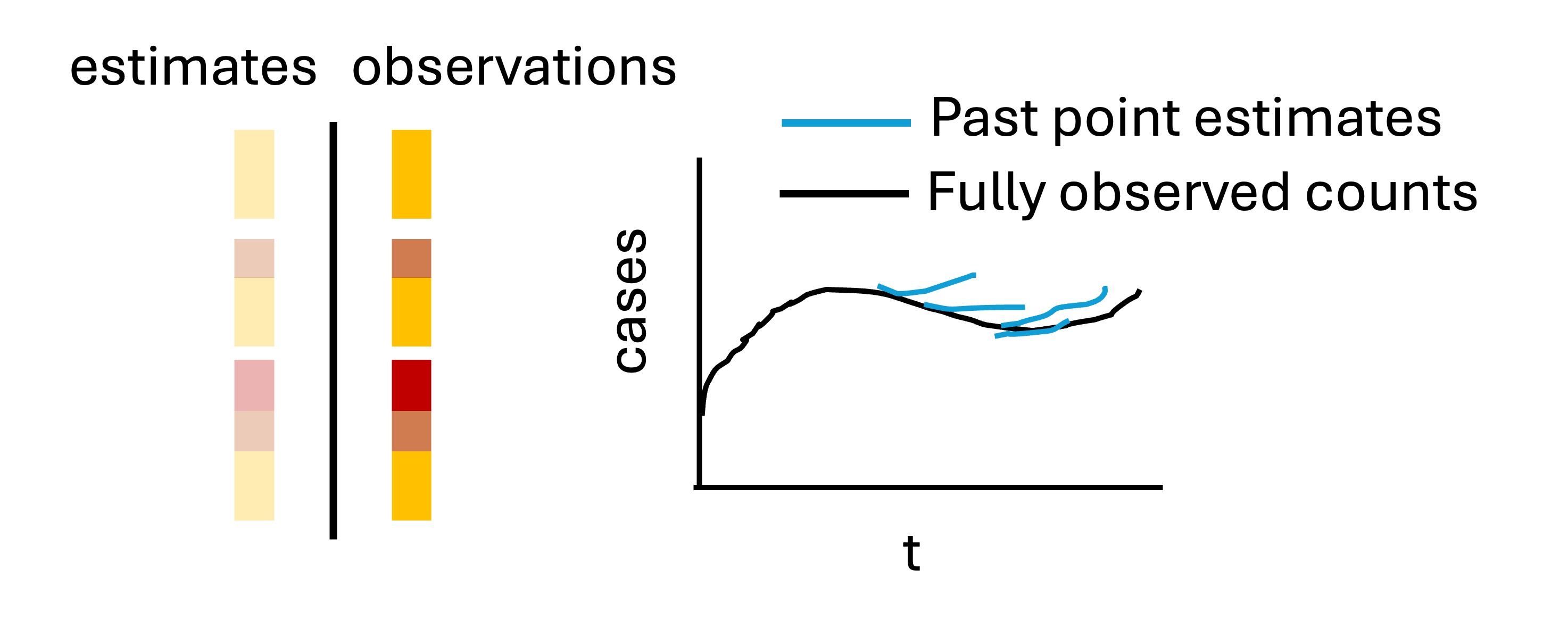
Figure 3: Visual description of the uncertainty quantification method, which generates retrospective point nowcasts and compares those estimates to what was later observed as of the nowcast time.
Probabilistic nowcast generation
Predicted probabilistic nowcast generation
Predictive distributions for \(X_{t^*}, \dots, X_{t^* - D + 1}\) are obtained by generating draws from the observation model, in this case a negative binomial, with the estimated dispersion parameters and a mean given by predicted component of the point nowcasts. Specifically, we set
\[ X_{t, > t^* - t} \sim \text{NegBin}(\hat{x}_{t, > t^* - t}, \phi_{t^* - t}). \] This is described in the schematic Figure 4 which depicts sampling from the observation model with a mean given by the sum of the predicted components in the point nowcast matrix (the shaded elements in the bottom right).
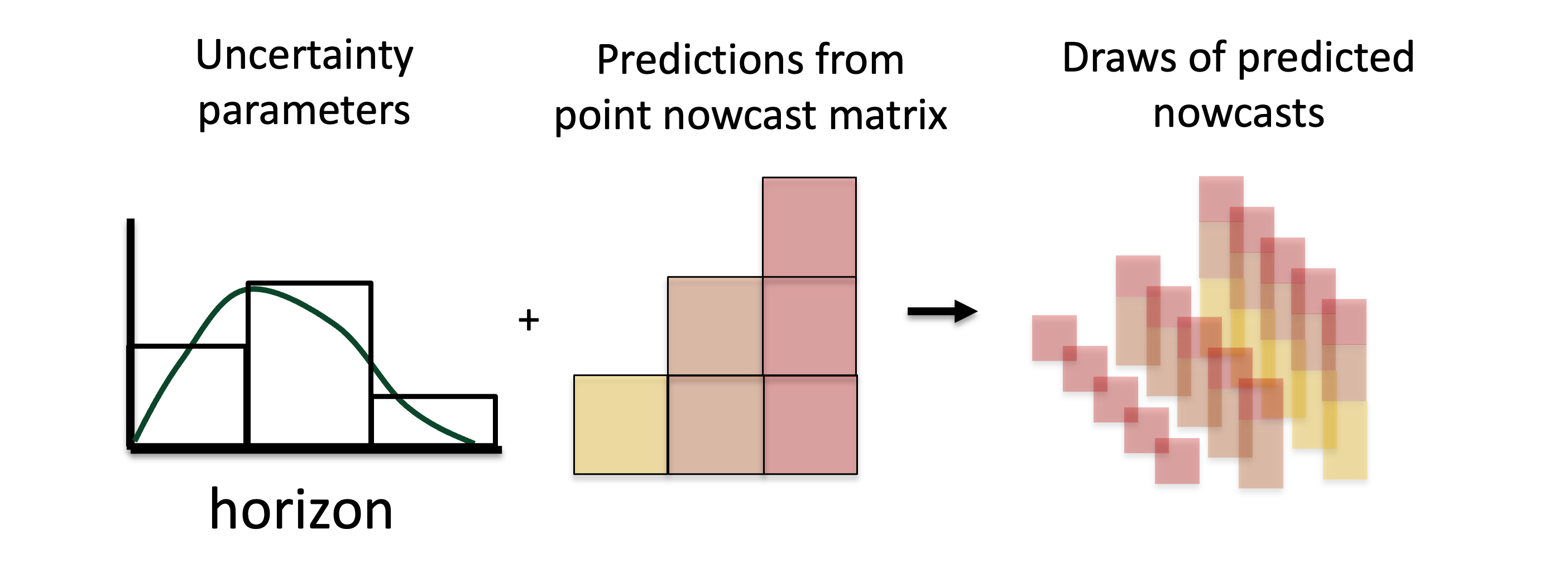
Figure 4: Visual description of the generation of predicted probabilistic nowcasts generated via sampling from the observation model with the estimated uncertainty parameters and a mean given by the sum of the predicted components at each reference time.
Combine with observations to obtain probabilistic nowcasts
The predictive distribution for \(X_{t}\) then results by shifting this distribution by the already known value \(x_{t, \leq t^* - t}\), or in other words adding the right-truncated partial observed data summed across reference times and the predicted probabilistic nowcast components to generate probabilistic nowcasts.
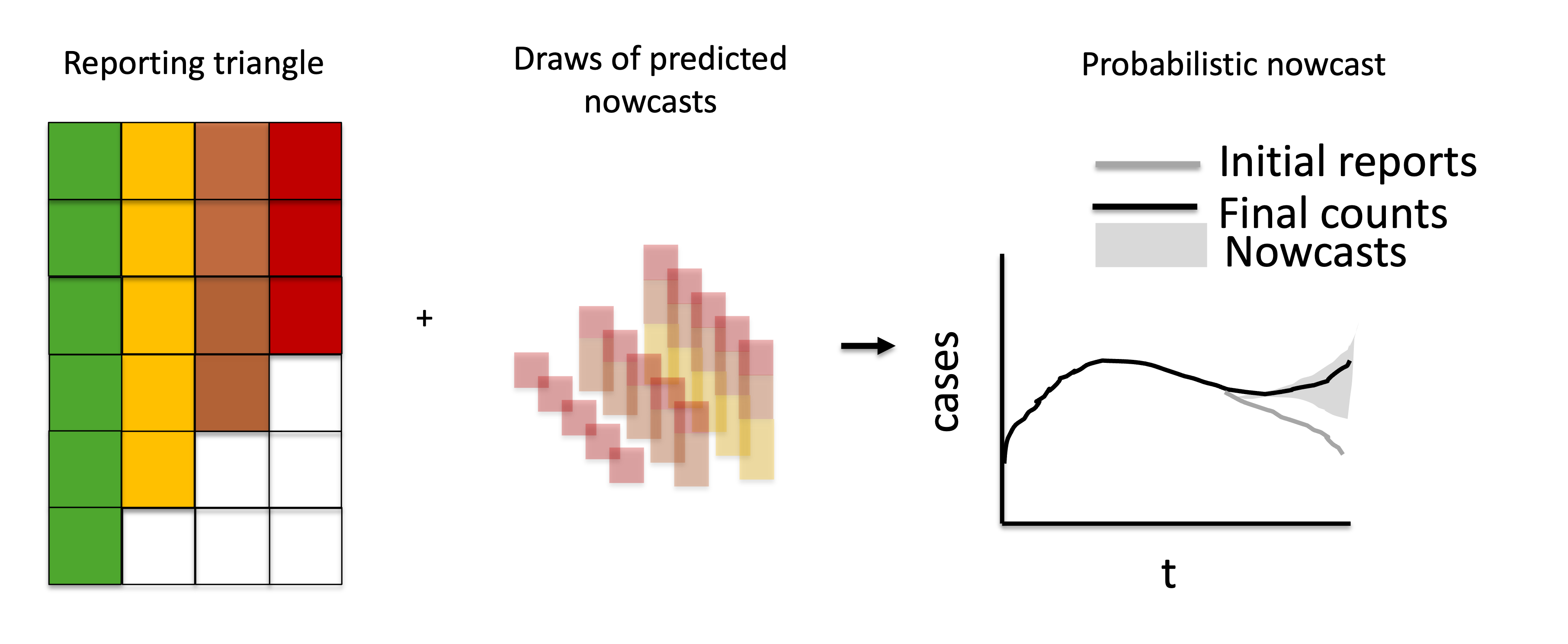
Figure 5: Visual description of combining the observations with the probabilistic predicted nowcast components to generate probabilistic nowcasts.
The sample_nowcasts() function ingests uncertainty parameters, the reporting triangle, and the point nowcast matrix and generates probabilistic nowcasts.
Zero-handling strategy
As mentioned in Point nowcast generation, we use a modified point nowcasts to deal with zero values in preliminary counts. We here motivate this approach from a Bayesian perspective, based on the work of[3]. To this end we assume that
\[ X_{t, \leq d} \ \mid X_t \sim \text{Bin}\left(X_t, \sum_{d = 0}^d \pi_t\right). \] We are now interested in the conditional expectation
\[ \mathbb{E}(X_t \ \mid X_{t, \leq d}) \]
in this binomial subsampling problem. We will derive it under the improper prior distribution
\[ X_t \sim \text{DiscreteUniform}(0, 1, 2, \dots). \]
For notational simplicity and readability for the following, we substitute \(N = X_{t}\), \(Y = X_{t, \geq d}\) and \(p = \sum_{d = 0}^D \pi_d\) and are thus looking for \(\mathbb{E}(N | Y = y)\) if \(Y \sim \text{Bin}(N, p)\) with a discrete uniform prior on \(N\). This expectation can be written out as: \[ \mathbb{E}(N \ | \ Y = y) = \sum_{n=0}^{\infty}\text{Pr}(N = n | Y = y) \times n (\#eq:expectation) \]
Applying Bayes Theorem we have \[ \text{Pr}(N = n \ |\ Y = y) = \frac{\text{Pr}(Y = y \ | \ N = n) \times \text{Pr}(N=n)}{\sum_{i=0}^{\infty}\text{Pr}( Y = y \ |\ N= i) \times \text{Pr}(N = i)}. \] Because \(\text{Pr}(N=n)\) is a constant this simplifies to \[ \text{Pr}(N = n \ |\ Y = y) = \frac{\text{Pr}(Y = y \ |\ N = n)}{\sum_{i=0}^{\infty}\text{Pr}( Y = y \ |\ N= i)}. \] Now substituting the probability mass function of the binomial distribution \[ \text{Pr}(Y = y\ |\ N = n) =\binom{n}{y} p^y(1-p)^{n-y} \] we get \[ \text{Pr}(N = n \ |\ Y = y) = \frac{\binom{n}{y} p^y(1-p)^{n-y}}{\sum_{i=1}^\infty \binom{1}{y}p^y(1-p)^{i-y}} \]
Plugging this into (??) we get the following (omitting terms for \(n<y\), which are 0):
\[ \mathbb{E}(N \ |\ Y = y) = \sum_{n=y}^{\infty}n \frac{\binom{n}{y} p^y(1-p)^{n-y}}{\sum_{i=y}^\infty \binom{i}{y}p^y(1-p)^{i-y}} \]
This is equivalent to
\[ \mathbb{E}(N \ | \ Y = y) = \frac{\sum_{n=y}^{\infty}n \binom{n}{y} p^y(1-p)^{n-y}}{\sum_{i=y}^\infty \binom{i}{y}p^y(1-p)^{i-y}}. \]
Both the numerator and the denominator are known convergent series, with solutions available in standard libraries like Mathematica[4]. We then get
\[ \mathbb{E}(N \ |\ Y = y) = \frac{(y + 1 -p)/p^2}{1/p} = \frac{y + 1 - p}{p}, \] which corresponds to the corrected point estimate provided in equation (5).
Default settings
To guide practitioners, we set default behaviours that are based on the maximum delay observed in the data. We use the partial reporting triangle for delay estimation, derive delay estimates and uncertainty estimates from only the reporting triangle being nowcasted, and use three times the maximum delay number (\(V=3 \times D\)) reference times for the total training volume \(V\) used by the model (in line with[1]).
Within each step there are additional defaults:
Delay distribution estimation: 50% of the reference times in the training volume \(V\) are used for delay estimation, \(N\), with a minimum requirement of at least one more than the maximum delay. If less data than this is available, this is indicated to the user, only producing an error when less data than the theoretically minimum is available for any given modelling step.
Point nowcast generation: Delay estimation occurs using the reporting triangle being nowcasted.
Uncertainty Estimation: 50% of the reference times in the training volume \(V\) are used as retrospective point nowcast times, \(M\). If there is insufficient data, the method uses the oldest retrospective nowcast date with at least the same amount of historical data for delay estimation as is used for the point nowcast at the current nowcast date, and requires that there are at least two retrospective nowcasts containing sufficient data. By default we do not sum the predicted components of each row across rows as this is context specific (diverging from[1]. who sum by week due to their target data being a rolling 7 day sum).